For quite a while, I’ve been confused by the behavior of the prop.test function in R: 1) the p-values always seem to be slightly off, and 2) the confidence intervals never seem to be symmetric around my estimate of the population proportion. Today, I decided I was going to figure out what was up… and whether I should trust my own analytical calculations for this test or what I get in R. I started by checking R Bloggers to see if anyone had explored this problem, but I only found one post about the two proportion z-test, and found none focusing on the one proportion z-test.
Here’s the essence of the test: you observe x subjects out of a sample size of n observations. Perhaps you just want to create a confidence interval to get a sense of where the true population proportion lies. Or maybe, you’d like to test the null hypothesis that the true population proportion is some value p0, against the alternative that it is really greater than, less than, or not equal to that value.
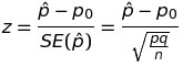
To do this, you can use the normal approximation to the binomial distribution to calculate a test statistic z. The estimated population proportion, p-hat, is just x/n. You have to find the standard error (SE) of your estimate as well to get the value of z:
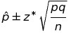
The confidence interval is constructed from the estimated population proportion, and the margin of error, which is determined by the standard error of the estimate and a scaling factor (z*) that establishes the width of the confidence interval:
![]()
![]()
 Here’s an example. Let’s say I know that nationally, 90% of home buyers would select a home with energy efficient features, even paying a premium of 2-3%, to reduce their utility costs long term. As the hypothetical president of an engineering firm that installs these energy efficient features, I want to know if less than 90% of buyers in my local area feel this way (because if so, I might want to launch an education campaign to help my business). I randomly sample 360 potential buyers and find that 312 of them would indeed select a home with energy efficient features.
I want to test my sample against the null hypothesis that the true population proportion is 0.90, with the alternative that the proportion is less than 0.90. I use a estimated population proportion (p-hat) of 312/360=0.867, and using the equations above, find that my test statistic z turns out to be -2.108, with a corresponding p-value of 0.0175. I reject the null hypothesis that the true population proportion is 0.90 in favor of the alternative, and start making plans to launch my education program.
(I don’t get the same values when I use prop.test. But later in this post, I’ll show you why I shouldn’t have expected that in the first place!!)
I wrote an R function to automate my z test (and also, to double check my calculations):
z.test <- function(x,n,p=NULL,conf.level=0.95,alternative="less") {
   ts.z <- NULL
   cint <- NULL
   p.val <- NULL
      phat <- x/n
      qhat <- 1 - phat
      # If you have p0 from the population or H0, use it.
      # Otherwise, use phat and qhat to find SE.phat:
      if(length(p) > 0) {
         q <- 1-p
         SE.phat <- sqrt((p*q)/n)
         ts.z <- (phat - p)/SE.phat
         p.val <- pnorm(ts.z)
         if(alternative=="two.sided") {
            p.val <- p.val * 2
         }
         if(alternative=="greater") {
            p.val <- 1 - p.val
         }
      } else {
      # If all you have is your sample, use phat to find
      # SE.phat, and don't run the hypothesis test:
         SE.phat <- sqrt((phat*qhat)/n)
      }
      cint <- phat + c(
         -1*((qnorm(((1 - conf.level)/2) + conf.level))*SE.phat),
         ((qnorm(((1 - conf.level)/2) + conf.level))*SE.phat) )
   return(list(estimate=phat,ts.z=ts.z,p.val=p.val,cint=cint))
}
When I run it on my example above, I get what I expect:
> z.test(312,360,p=0.9)
$estimate
[1] 0.867

$ts.z
[1] -2.11

$p.val
[1] 0.0175

$cint
[1] 0.836 0.898
But when I run prop.test, this isn’t what I see at all!
> prop.test(312,360,p=0.9)

 1-sample proportions test with continuity correction

data: 312 out of 360, null probability 0.9
X-squared = 4.08, df = 1, p-value = 0.04335
alternative hypothesis: true p is not equal to 0.9
95 percent confidence interval:
 0.826 0.899
sample estimates:
 p
0.867
Why are there differences? Here’s what I found out:
- The prop.test function doesn’t even do a z test. It does a Chi-square test, based on there being one categorical variable with two states (success and failure)! Which I should have noticed immediately from the line that starts with “X-squared” 🙂
- The Yates continuity correction, which adjusts for the differences that come from using a normal approximation to the binomial distribution, is also automatically applied. This removes 0.5/n from the lower limit of the confidence interval, and adds 0.5/n to the upper limit.
- Most notably, I was really disturbed to see that the confidence interval given by prop.test wasn’t even centered around the sample estimate, p-hat. Oh no! But again, this is no concern, since prop.test uses the Wilson score interval to construct the confidence interval. This results in an asymmetric, but presumably more accurate (with respect to the real population) confidence interval.
Moral of the story? There are many ways to test an observed proportion against a standard, target, or recommended value. If you’re doing research, and especially if you’re using R, be sure to know what’s going on under the hood before you report your results.
(Other moral? Try binom.test.)


Leave a Reply