The Central Limit Theorem (CLT), and the concept of the sampling distribution, are critical for understanding why statistical inference works. There are at least a handful of problems that require you to invoke the Central Limit Theorem on every ASQ Certified Six Sigma Black Belt (CSSBB) exam. The CLT says that if you take many repeated samples from a population, and calculate the averages or sum of each one, the collection of those averages will be normally distributed… and it doesn’t matter what the shape of the source distribution is! (Caveat: so long as the data comes from a distribution with finite variance… so that means the Cauchy distribution doesn’t count.)

I wrote some R code to help illustrate this principle for my students. This code allows you to choose a sample size (n), a source distribution, and parameters for that source distribution, and generate a plot of the sampling distributions of the mean, sum, and variance. (Note: the sampling distribution for the variance is a Chi-square distribution — if your source distribution is normal!)

sdm.sim <- function(n,src.dist=NULL,param1=NULL,param2=NULL) {
   r <- 10000  # Number of replications/samples - DO NOT ADJUST
   # This produces a matrix of observations with  
   # n columns and r rows. Each row is one sample:
   my.samples <- switch(src.dist,
	"E" = matrix(rexp(n*r,param1),r),
	"N" = matrix(rnorm(n*r,param1,param2),r),
	"U" = matrix(runif(n*r,param1,param2),r),
	"P" = matrix(rpois(n*r,param1),r),
        "B" = matrix(rbinom(n*r,param1,param2),r),
	"G" = matrix(rgamma(n*r,param1,param2),r),
	"X" = matrix(rchisq(n*r,param1),r),
	"T" = matrix(rt(n*r,param1),r))
   all.sample.sums <- apply(my.samples,1,sum)
   all.sample.means <- apply(my.samples,1,mean)   
   all.sample.vars <- apply(my.samples,1,var) 
   par(mfrow=c(2,2))
   hist(my.samples[1,],col="gray",main="Distribution of One Sample")
   hist(all.sample.sums,col="gray",main="Sampling Distribution\nof
	the Sum")
   hist(all.sample.means,col="gray",main="Sampling Distribution\nof the Mean")
   hist(all.sample.vars,col="gray",main="Sampling Distribution\nof
	the Variance")
}

There are 8 population distributions to choose from: exponential (E), normal (N), uniform (U), Poisson (P), binomial (B), gamma (G), Chi-Square (X), and the Student’s t distribution (T). Note also that you have to provide either one or two parameters, depending upon what distribution you are selecting. For example, a normal distribution requires that you specify the mean and standard deviation to describe where it’s centered, and how fat or thin it is (that’s two parameters). A Chi-square distribution requires that you specify the degrees of freedom (that’s only one parameter). You can find out exactly what distributions require what parameters by going here: http://en.wikibooks.org/wiki/R_Programming/Probability_Distributions.

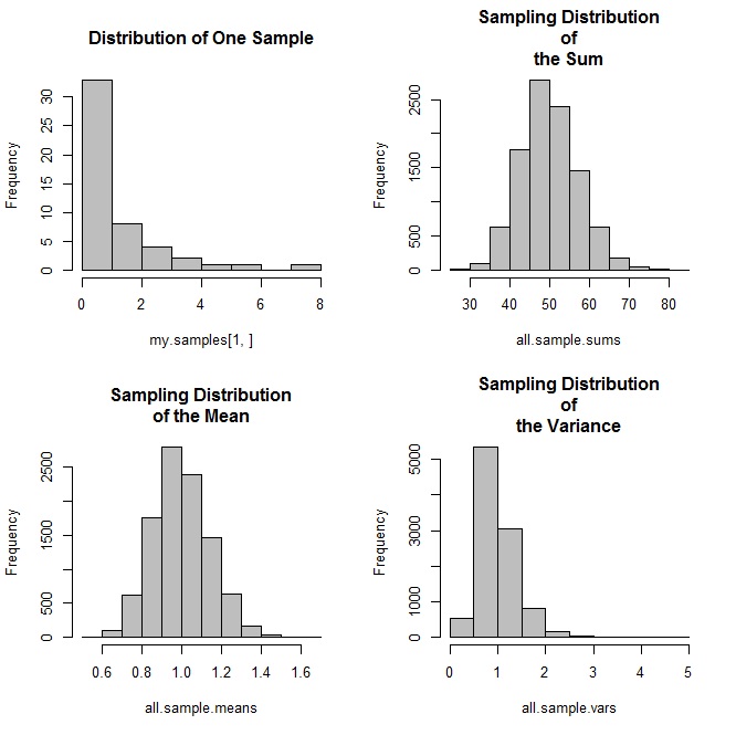
Here is an example that draws from an exponential distribution with a mean of 1/1 (you specify the number you want in the denominator of the mean):

sdm.sim(50,src.dist="E",param1=1)

The code above produces this sequence of plots:

sd-blog-1

You aren’t allowed to change the number of replications in this simulation because of the nature of the sampling distribution: it’s a theoretical model that describes the distribution of statistics from an infinite number of samples. As a result, if you increase the number of replications, you’ll see the mean of the sampling distribution bounce around until it converges on the mean of the population. This is just an artifact of the simulation process: it’s not a characteristic of the sampling distribution, because to be a sampling distribution, you’ve got to have an infinite number of samples. Watkins et al. have a great description of this effect that all statistics instructors should be aware of. I chose 10,000 for the number of replications because 1) it’s close enough to infinity to ensure that the mean of the sampling distribution is the same as the mean of the population, but 2) it’s far enough away from infinity to not crash your computer, even if you only have 4GB or 8GB of memory.

Here are some more examples to try. You can see that as you increase your sample size (n), the shapes of the sampling distributions become more and more normal, and the variance decreases, constraining your estimates of the population parameters more and more.

sdm.sim(10,src.dist="E",1)
sdm.sim(50,src.dist="E",1)
sdm.sim(100,src.dist="E",1)
sdm.sim(10,src.dist="X",14)
sdm.sim(50,src.dist="X",14)
sdm.sim(100,src.dist="X",14)
sdm.sim(10,src.dist="N",param1=20,param2=3)
sdm.sim(50,src.dist="N",param1=20,param2=3)
sdm.sim(100,src.dist="N",param1=20,param2=3)
sdm.sim(10,src.dist="G",param1=5,param2=5)
sdm.sim(50,src.dist="G",param1=5,param2=5)
sdm.sim(100,src.dist="G",param1=5,param2=5)

18 responses to “Sampling Distributions and Central Limit Theorem in R”

  1. Top 10 Statistics Topics for the Six Sigma Black Belt (CSSBB) Exam | Quality and Innovation Avatar

    […] Central Limit Theorem – This is the magic that serves as the foundation for so much of what quality professionals practice. In short, whenever you take many samples for which you have a sum or an average value that you’ve computed over that sample, the distribution of the whole collection of sums or means is going to be normal!! This is why when we’re spot checking parts or products in quality control, we take batch averages and know they’re going to be distributed normally. Find out more here! […]

  2. Ray Jones Avatar
    Ray Jones

    Greta article – loved playing with the code. Can you point me at where you got this bit from: “Note: the sampling distribution for the variance is a Chi-square distribution!” – I’m trying to verify this myself in a document I’m producing and I just can’t get the variances to look chi-squared from some of the distributions (uniform for example). I’ve looked hard at Cochran’s Theorem and convinced myself this would not apply to the variances directly computed from the random samples but only to samples of the means of those random samples. If you could point me to a more formal description of why you would expect the variances of the random samples to be chi-squared distributed it’d be very helpful to me. Thanks.

    1. Nicole Radziwill Avatar
      Nicole Radziwill

      Hi Ray! Here’s a nice, straightforward explanation of the “sampling distribution of the variance is a Chi-square”… https://onlinecourses.science.psu.edu/stat414/node/174 — if you have any insight into the subtleties, I’d love to hear about them. I’m always learning and looking for new opportunities to get a deeper understanding of stuff.

      Glad you had fun playing with the code too 🙂

      1. Ray Jones Avatar
        Ray Jones

        Thanks for the quick response and the link – what it says is:

        “Theorem. Suppose:

        X1, X2, … , Xn are observations of a random sample of size n from the normal distribution N(μ, σ2) ”

        Problem is that if the pdf generating the random sample is uniform (say) then the X1, X2 etc. are not a “random sample from the normal distribution..”. I just spent 3-4 days banging my head on this – I found Cochran’s Theorem (which is what your link is talking about) and I initially misinterpreted it (I think) and then spent a few days trying to show that the variances from a random sample from a uniform pdf are chi-squared distributed. I also just tried it with your code – have a go with a uniform distribution between -2 & +2 and you’ll see my problem.

        What I finally convinced myself of, is that, since the CLT says the means of random samples will be normally distributed, then Cochran’s Theorem says the variances of samples of the means of random samples will be chi-squared distributed – as they are shown to be in my paper that I am putting together (see https://rpubs.com/ray_jones/69849 for the state of the current draft). What you’ll see in my code is that I had to do an extra step – once I have the array of means of the random samples then I have to do a bootstrap to generate an array of variances from sub-sets of the means.

        Cutting a long story short – I don’t think the link you give is saying what you think it is – but I’ll be very happy if you can tell me where I am wrong.

        Thanks

        Ray

      2. Nicole Radziwill Avatar
        Nicole Radziwill

        So I ran the case of the sim you were talking about and yeah… doesn’t look Chi-square at all. And I think you’re right, you can’t interpret the link I provided as being accurate for anything other than a normal source distribution. I found this from some MIT online courseware: “Unfortunately there is no CLT analog for variance… But there is an important special case, which is when X1, X2, . . . , Xn are from a normal distribution. (Recall that the CLT applies to arbitrary distributions.)” (from http://ocw.mit.edu/courses/sloan-school-of-management/15-075j-statistical-thinking-and-data-analysis-fall-2011/lecture-notes/MIT15_075JF11_chpt05.pdf) — have to go read your paper/code, haven’t done that yet. But this is definitely on my mind now…

  3. Ray Jones Avatar
    Ray Jones

    My advice is to try not to bang your head on this quite as much as I did ….

    1. Nicole Radziwill Avatar
      Nicole Radziwill

      Maybe someone else will chime in and head us off at the pass 🙂

  4. Ray Jones Avatar
    Ray Jones

    Hello again – sorry to be the bearer of bad tidings (again) but you have another issue with your code. I know this because I’ve just implemented the Cauchy distribution in my report and had the same problem. Strictly speaking the Cauchy does not obey the CLT because it is not a finite distribution. In order to make it finite you have to impose a cutoff threshold. The way this manifests in your charts is that for the Cauchy you’ll see truly enormous outliers that ruin the scaling – this is not strictly speaking incorrect since they are genuine random samples from the distribution but it does make it impossible to see what you’re trying to show, i.e. that the CLT holds for most of the random samples. In my report I just imposed a threshold like this:
    “`
    sample cutoff] <- location
    “`

  5. Ray Jones Avatar
    Ray Jones

    Ooops – sorry that didn’t work. My code looks like this:
    sample cutoff] <- location

    1. Nicole Radziwill Avatar
      Nicole Radziwill

      Hi Ray – no bad news/bad tidings at all – this is what I love about blogging and connecting with people. I’m going to take Cauchy out of the mix because of https://www.ma.utexas.edu/users/mks/M358KInstr/Cauchy.pdf — yet another special case!! Apparently due to infinite variance.

      1. Ray Jones Avatar
        Ray Jones

        You may find you have the same issue with Student t – that can also be undefined in mean and variance – I haven’t got to that one yet but I imagine i’ll handle it in the same way – i.e. make it finite by imposing a cutoff threshold in x.

  6. Ray Jones Avatar
    Ray Jones

    Still didn’t work – last time I’ll try:

    sample cutoff] <- location

    1. Ray Jones Avatar
      Ray Jones

      So I finished the first draft of my paper [here](https://rpubs.com/ray_jones/69849) – when I did the Student’s t it turns out that provided you use a value of nu > 2 then the variance is defined but I still had the problem with the outliers messing up the scaling on the plots – so I ended up implementing a cutoff threshold anyway. I had a go with your code and your Student’s t has the same problem – the plots get messed up by the outliers.

  7. Miodrag Avatar
    Miodrag

    Hi Ray and Nicole. (n-1) * Sampling variance/ (Population variance) follows Chi-square distribution with n-1 df only when the population is normal. If the population is not normal s.d. of sampling variance does not follow chi-square. Ray, I spent one hour to find bugs in your code. What have you done is to wrongly produce the distribution of sampling variance using the means! For all of your distributions, you should have added a line SampleVariance <- c(SampleVariance, var(sample) immediately following the line in which you drew samples. Only then you would see that the distribution of sample variances tend to follow the normal distribution when the sample is large, NOT the chi-square! Of course, this does not apply to the Cauchy distribution. Anyway, Nicole has mad a terrific simulation of the CLT, short and powerful.

  8. Miodrag Avatar
    Miodrag

    You can find a nice video about this https://www.youtube.com/watch?v=V4Rm4UQHij0

  9. Object of Type Closure is Not Subsettable ⋆ Quality and Innovation Avatar

    […] take something that’s very obviously a function. I picked the sampling distribution simulator from a 2015 blog post I wrote. Cut and paste it into your R […]

  10. […] take something that’s very obviously a function. I picked the sampling distribution simulator from a 2015 blog post I wrote. Cut and paste it into your R […]

Leave a Reply

I’m Nicole

Since 2008, I’ve been reflecting on Digital Transformation & Data Science for Performance Excellence here. As a CxO, I’ve helped orgs build empowered teams, robust programs, and elegant strategies bridging data, analytics, and artificial intelligence (AI)/machine learning (ML)… while building models in R and Python on the side. In 2024, I help leaders navigate the complex market of data/AI vendors & professional services. Need help sifting through it all? Reach out to inquire.

More About Me or Inquire @ Engaging a Team

Let’s connect